
Analysis of Police Activity in Madison, WI : Using Speech-to-text Decoding for P25 Police Radio
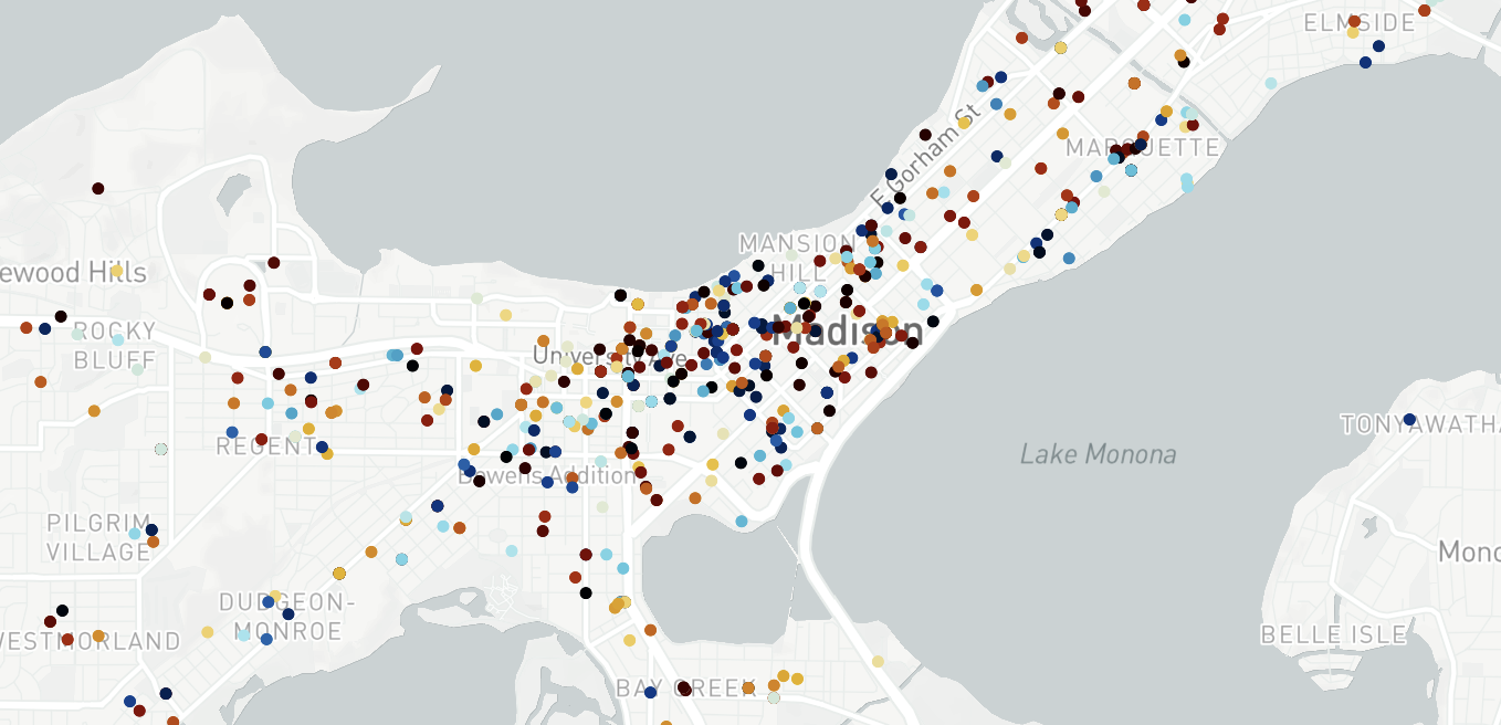
Hover and zoom [top right controls] into graph for more information. Addresses extracted from Madison PD P25 voice channels from 10/18/22 to 11/10/22. Color scale corresponding to hour of day the address was mentioned.
Intro
With the recent introduction of OpenAI’s Whisper transformer based speech-to-text model, I became interested with the real-world applications given its human-level interpretation of spoken language.
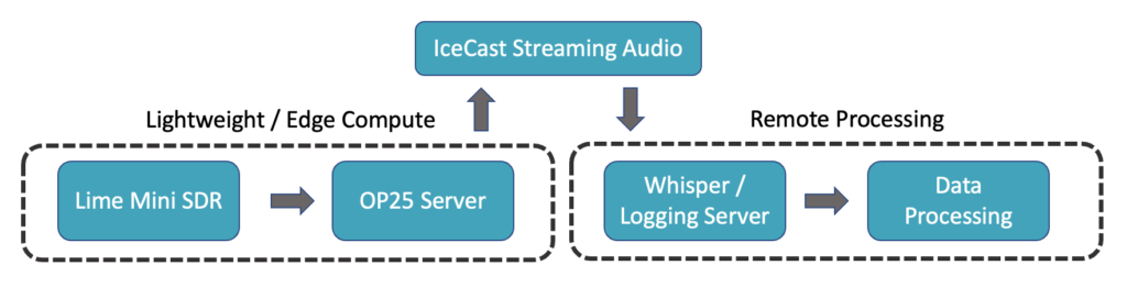
Combining two of my interests, machine learning and radios, I focused in on P25 trunked radio systems – commonly used by police districts for communication. At a high-level, I was interested in developing an abstract system that was separated into three parts:
- Hardware level P25 decoding into voice
- Preferably on the edge to support inaccessible antenna locations
- Multi-processed software to cache streamed voice data and jointly convert into textual data using Whisper
- As output have organized, time-stamped textual data
- Hands-off data analysis for generating comprehensible graphs and metrics surrounding the local police department
Although the project is still in development, I have come to a point where enough interesting information exists, warranting my first blog post.
As a side note, decoding unencrypted police radio is entirely legal. There exist numerous websites allowing you to stream police radio from all over the United States. I chose to implement this project end-to-end both to have complete control over what was being decoded and to increase decoding quality. Overall, the goal of the project centered around making this public information more publicly available through straightforward analysis.
Hardware
Starting off with the radio itself, I chose a LimeSDR Mini from Lime Microsystem. Paired with the radio was a Bingfu UHF antenna tuned to cover 850 MHz. For processing, I used an Intel i5 NUC for both decoding P25 transmissions and running Whisper. Data analysis was done on an M1 Macbook.
Software
SoapySDR: Platform neutral SDR support for interacting with Lime SDR
OP25: P25 signal decoding and IceCast audio streaming
Google Geolocation API: Address to latitude/longitude conversion
Plotly: Visualizations
P25 Decoding
For a general overview, P25 is broken into various “phases”. The most common used modulations are Phase 1 and Phase 2:
- Phase 1:
- 9600bps
- either C4FM or CQPSK modulations
- Phase 2:
- 12000bps
- TDMA modulations
P25 transmissions may also be digitally encrypted using standards such as Advanced Encryption Standard (AES), U.S. Data Encryption Standard (DES), as well as others. To support encryption, specifications exist in the P25 standard for over-the-air rekeying to update keys across a network. Fortunately, the local Madison police department is largely unencrypted allowing transmissions to be decoded.
P25 systems also carry a Network Access Code (NAC) and Talkgroup ID with each transmission. The NAC specifies which trunked system the radio is connected to while the Talkgroup ID allows traffic to be subdivided into various categories. For my use case in Madison, there were two options for systems: DaneCom (P25 Phase II) and Madison Public Safety (P25 Phase I). Given my proximity to downtown Madison I chose to monitor the Madison Public Safety system which includes Madison PD, University of Wisconsin PD, and Capitol PD.
In the next section I show how to source local frequency details and setup OP25.
Sourcing Frequencies and OP25
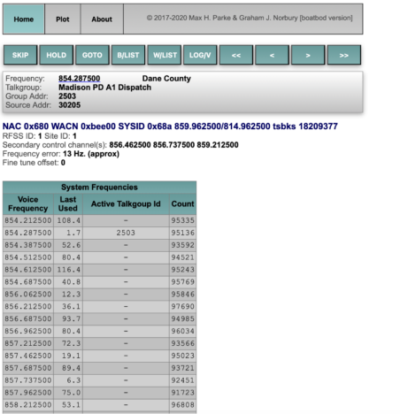
RadioReference is your friend here, use it to both explore the various systems in use nearby and use it also for extracting control frequencies and Talkgroup ID → channel description mappings. For example, here lists all the FCC licensed frequencies in Madison, WI. Going deeper, this is a list specific to Madison Public Safety system.
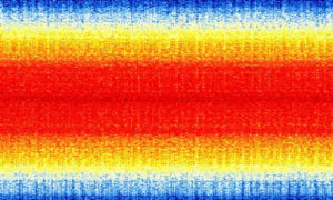
Moving to OP25, the setup is fairly simple. Given the Lime SDR is not natively supported by OP25, we have to work with SoapySDR to provide an abstraction for the hardware – setup instructions linked above. Lastly, before jumping into decoding voice, I suggest using SDR software (SDRPlusPlus is a great option) to visualize control frequencies and ensure you are physically able to read the signal. An example of P25 on a spectrum waterfall is shown below.
To allow remote streaming of the voice channel, we will use IceCast. Setup instructions for IceCast located in the apps directory: op25/gr-op25_repeater/apps/README
Use the ./rx script to run OP25: python3 ./rx.py --args 'driver=lime,soapy=0' --gains 'lna:47' -f 859.9625e6 -o 17e3 -S 5000000 -q 0 -w -2 -l http:192.168.86.25:8002 -T trunk.tsv -M meta.json -V
As a last decoding step I implemented a whitelist for OP25 to only listen to select call channels.
These channels were:
-
-
- Madison PD A1 Dispatch
- Madison PD A3 Dispatch
- Madison PD A7 Tactical
- Madison PD A8 Tactical
- Capitol Police – Main
- Capitol Police – Tac
- UWPD Main
- UWPD TAC
-
Audio-to-text Translation
For converting audio to text, a small multi-processed program was used for both buffering the streaming audio into memory, and then processing the block using Whisper and Pandas.
Whisper takes in 30 second chunks of audio sampled at 16kHz, therefore I used ffmpeg to extract buffers of this size and store in a shared queue. The Whisper process consumes these buffers and runs the pre-trained, size small, English-specific, Whisper model. Surprisingly, running a single forward pass of the transformer on an outdated i5 CPU took only around 5 seconds on average (6x faster than real-time). To avoid running Whisper on empty frames, the buffer’s Mel Spectrogram needed to exceed a noise floor of a prespecified value in order to run. Lastly, the outputted textual data is timestamped and appended to a Pandas dataframe which is then saved to a CSV every hundred entries.
# Gabriel Gozum 2022
import whisper
import ffmpeg
import numpy as np
import pandas as pd
import torch
import time
from datetime import datetime
from multiprocessing import Process
from multiprocessing import Queue

# constants
FS              = 16000
BUFFER_SIZE     = FS*60
NOISE_FLOOR     = -1.5
INT_16_MAX_F    = 32768.0

def ffmpeg_process(url, q, debug=True):
    process = (
        ffmpeg.input(url)
        .output("-", format='s16le', acodec='pcm_s16le', ac=1, ar=FS, loglevel="quiet")
        ).run_async(pipe_stdout=True)

    while True:
        if debug:
            start = time.time()
        in_bytes = process.stdout.read(BUFFER_SIZE)
        out = np.frombuffer(in_bytes, np.int16).flatten().astype(np.float32) / INT_16_MAX_F

        if debug:
            stop = time.time()
            print(f"ffmpeg time: {stop - start}")

        q.put(out)


def whisper_process(q, debug=True):
    model = whisper.load_model("small.en")
    options = whisper.DecodingOptions(language="en", without_timestamps=True, fp16=False)

    save_location = f'./data/csv/{datetime.now().strftime("%d_%m_%y_%H_%M")}.csv'
    df = pd.DataFrame(columns=['time', 'text'])

    while(True):
        out = q.get()

        if debug:
            start = time.time()

        audio = whisper.pad_or_trim(out)
        mel = whisper.log_mel_spectrogram(audio).to(model.device)

        # skip empty clips
        if (torch.max(mel) <= NOISE_FLOOR):
            continue

        result = whisper.decode(model, mel, options)

        df.loc[len(df.index)] = [datetime.now().strftime("%H:%M:%S %d/%m/%Y"), result.text]

        if len(df.index) % 100 == 0:
            df.to_csv(save_location)
            save_location_new = f'./data/csv/{datetime.now().strftime("%d_%m_%y_%H_%M")}.csv'
            if save_location != save_location_new:
                df = pd.DataFrame(columns=['time', 'text'])
                save_location = save_location_new

        if debug:
            stop = time.time()
            print(f"length of dataframe: {len(df.index)}")
            print(f"whisper time: {stop - start}", flush=True)
            print(result.text, flush=True)


def main():
    q = Queue()

    # ffmpeg sampling
    p1 = Process(target=ffmpeg_process, args=("http://localhost:8001/op25", q,))
    p1.start()

    # whisper processing / logging
    p2 = Process(target=whisper_process, args=(q,))
    p2.start()

    # cleanup (never hits)
    p1.join()
    p2.join()


if __name__ == "__main__":
    main()
Analysis
In total, the entire radio and logging process ran for three weeks generating 50,000 time-stamped textual entries. There were multiple metrics I was interested in extracting from this data – namely studies on described race and mapping areas of high police activity. For this blog post I will only be presenting results concerning police activity in Madison, WI.
Mapping
Starting out, I need a method to extract addresses from text. Surprisingly I could not find a pre-existing NLP or deep-learning based approach for this. Given more time I would have looked into training a lightweight model off a dataset with labeled addresses (Name Entity Recognition with custom spaCy model); however, given this is just a blog and I am a PhD student, my fall-back solution was regex statements. Visibly looking at addresses called out, I found two common address types used by the police:
- Addresses starting with numbers, then containing names, and ending with “street/place/road/lane”
- Addresses at intersections, i.e. “intersection of State and Lake”
Using regex statements that captured these locations, I manually verified this approach with a day’s worth of text and achieved 86% accuracy without any false positives (pretty good 🤠). Another approach I explored was comparing the textual data against a large set of street names in Madison; however, I found this approach to not be scalable and I also ran into problems with street names overlapping with suspect names.
| time | address | data | ||
| 00:30:43 01/11/2022 | State Street | I’m out on State Street and you can change this to a [redacted]. 1230 that’s gonna be for an adult right? | ||
| 00:32:40 01/11/2022 | State Street | You can put me on State Street. | ||
| 00:35:14 01/11/2022 | Kelly Street | Frank 11 I got your call now it’s gonna be on Kelly Street. | ||
| 00:52:43 01/11/2022 | 501 West Main Street | David 10 David 2 assist citizen 501 West Main Street. | ||
| 02:03:06 01/11/2022 | Ohio Street | Last night on Ohio Street, an incident occurred that the caller would like to talk. |
Coordinate Extraction and Visualization
With the given addresses listed in Madison, I needed to cross reference these intersections and street names to known latitude and longitude coordinates. Luckily Google has a slick Geocode API that does just that – I combined this with an open source python library named geopy to append a column to my dataframe which contained full locations for the addresses. I chose Plotly for the visualizations given it harmonizes well with dataframes and has support for MapBox. I decided to color code the individual locations by time of day (24 hour scale), adding another element to the analysis.
Conclusion
In summary, the interactive map at the top visualizes the final results for this project. I found it enjoyable to cross reference thing such as business names with extracted addresses as a final form of verification. Also, there are fun correlations that are somewhat visible with the color coding. Stereotypical freshman bars have late-night police calls for intoxication and as expected, State Street is lined with calls occurring at all times of day.
There are many data-collection improvements and advances to the analysis that are in the works; however, interesting results exist in the current state. The SDR is still logging information to this day, I look forward to growing the dataset and improving analytics – but for now I need to focus back on being a PhD student.
P.S. The script above works with any Broadcastify police stream, just point it to the location and begin logging data.